OpenVINO™工具組能快速部署模擬人類視覺的應用程式和解決方案。此工具組將電腦視覺 (CV) 工作負載延伸至採用 Convolutional Neural Network (CNN) 的 Intel® 硬體,將效能最大化。這些步驟通常遵循本文中關於 Intel® 類神經電腦棒 2與開放原始碼OpenVINO™工具組,但包含特定的變更,讓所有內容在主機板上執行。
下載原始碼與安裝依存關係
| 注意 |
我們建議在從 openvinotoolkit GitHub 頁面的儲存庫中,指定最新且穩定的分支或標籤,而不是預設直接重做主分支。 |
Intel® OpenVINO™工具組的開放原始碼版本可透過 GitHub 取得。存放庫資料夾是格 溫特的 openvino。
cd ~/
git clone –recurse-submodules –single-branch –branch=2022.1.0 https://github.com/openvinotoolkit/openvino.git
Intel® OpenVINO™工具組有許多建置依存關係。install_build_dependencies.sh 腳本可為您取用。如果嘗試執行腳本時出現任何問題,您必須單獨安裝每個依存度。
執行腳本以安裝 Intel® OpenVINO™工具組的依存關係:
cd openvino
sed -i ‘s/raspbian/debian/g’ install_build_dependencies.sh
sudo ./install_build_dependencies.sh
如果腳本完成成功,您已準備好建置工具組。如果目前發生故障,請確保安裝任何列出的依存關係,然後再試一次。
建築
若要建立 Python API 包裝,請安裝以下所列的所有額外套件:
python3 -m pip install –upgrade pip
python3 -m pip install clang==11.0 pyaml
python3 -m pip install -r ~/openvino/src/bindings/python/src/compatibility/openvino/requirements-dev.txt
python3 -m pip install -r ~/openvino/src/bindings/python/wheel/requirements-dev.txt
| 注意 |
使用 -DENABLE_PYTHON=ON 選項。若要指定確切的 Python 版本,請使用下列選項:
-DPYTHON_EXECUTABLE=`which python3.9` \
-DPYTHON_LIBRARY=/usr/lib/aarch64-linux-gnu/libpython3.9.so \
-DPYTHON_INCLUDE_DIR=/usr/include/python3.9
使用 -DCMAKE_INSTALL_PREFIX={BASE_dir}/openvino_dist 指定 CMake 大樓要建置的目錄:
舉例來說, -DCMAKE_INSTALL_PREFIX=~/openvino_dist |
該工具組使用 CMake 建物系統來引導並簡化建物流程。若要為Intel® 類神經電腦棒 2打造推斷引擎和 MYRIAD 外掛程式,請使用下列命令:
| 注意 |
執行以下命令時,請移除所有的背擊 (\)。反沖用於通知這些命令未分離。 |
cd ~/openvino
mkdir build && cd build
cmake -DCMAKE_BUILD_TYPE=Release \
-DCMAKE_INSTALL_PREFIX=~/openvino_dist \
-DENABLE_INTEL_MYRIAD=ON \
-DENABLE_INTEL_CPU=OFF \
-DENABLE_INTEL_GPU=OFF \
-DENABLE_CLDNN=OFF \
-DENABLE_AUTO=OFF \
-DENABLE_MULTI=OFF \
-DENABLE_HETERO=OFF \
-DENABLE_TEMPLATE=OFF \
-DENABLE_TESTS=OFF \
-DENABLE_OV_ONNX_FRONTEND=OFF \
-DENABLE_OV_PADDLE_FRONTEND=OFF \
-DENABLE_OV_TF_FRONTEND=OFF \
-DENABLE_NCC_STYLE=OFF \
-DENABLE_SSE42=OFF \
-DTHREADING=SEQ \
-DENABLE_OPENCV=OFF \
-DENABLE_PYTHON=ON \
-DPYTHON_EXECUTABLE=$(which python3.9) \
-DPYTHON_LIBRARY=/usr/lib/aarch64-linux-gnu/libpython3.9.so \
-DPYTHON_INCLUDE_DIR=/usr/include/python3.9 ..
make -j4
sudo make install
如果由於 OpenCV 程式庫的問題而 發出 命令失敗,請確定您已告知系統您的 OpenCV 安裝地點。如果目前完成建置,Intel® OpenVINO™工具組已準備好執行。請注意,建置位於 ~/openvino/bin/aarch64/Release 資料夾中。
驗證安裝
成功完成推斷引擎組建後,您應確認所有裝置都已正確設定。若要確認工具組與Intel® 類神經電腦棒 2在您的裝置上運作,請完成下列步驟:
- benchmark_app執行範例程式,確認所有程式庫載入正確。
- 下載 經過訓練的型號。
- 選 取類神經網路的輸入。
- 設定 Intel® 類神經電腦棒 2 Linux* USB 驅動程式。
- 使用所選的型號和輸入執行object_detection_sample_ssd。
範例應用程式
Intel® OpenVINO™工具組包含一些使用推斷引擎與Intel® 類神經電腦棒 2的範例應用程式。其中一個程式 是benchmark_app, 可在下列專案中找到:
~/openvino/bin/aarch64/Release
執行下列命令以測試 benchmark_app:
cd ~/openvino/bin/aarch64/Release
./benchmark_app -h
它應該會列印說明對話,說明計畫的可用選項。
下載模型
該計畫需要一個模型來傳遞輸入。您可以取得以® IR 格式OpenVINO™工具組的模型:
- 使用 Model Optimizer 將現有模型從支援的框架之一轉換為推斷引擎的 IR 格式
- 使用 Model Downloader 工具從 Open Model Zoo 下載
- 直接從 storage.openvinotookit.org 下載 IR 檔案
就我們而言,直接下載最簡單。使用下列命令來取得人車單車偵測模型:
cd ~/Downloads
wget https://storage.openvinotoolkit.org/repositories/open_model_zoo/2022.1/models_bin/3/person-vehicle-bike-detection-crossroad-0078/FP16/person-vehicle-bike-detection-crossroad-0078.bin
wget https://storage.openvinotoolkit.org/repositories/open_model_zoo/2022.1/models_bin/3/person-vehicle-bike-detection-crossroad-0078/FP16/person-vehicle-bike-detection-crossroad-0078.xml
| 注意 |
Intel® 類神經電腦棒 2需要針對 16 位浮點格式(稱為 FP16)優化的模型。如果您的模型與範例不同,可能需要使用 Model Optimizer 轉換為 FP16。 |
神經網路的輸入
最後需要的專案是神經網路的輸入。對於我們下載的型號,您需要具有 3 個色彩通道的影像。將必要的檔案下載到主機板:
cd ~/Downloads
wget https://cdn.pixabay.com/photo/2018/07/06/00/33/person-3519503_960_720.jpg -O person.jpg
設定Intel® 類神經電腦棒 2 Linux USB 驅動程式
需要新增一些 udev 規則,使系統能夠辨識Intel® NCS2 USB 裝置。
| 注意 |
如果目前的使用者不是使用者群組的成員,請執行下列命令並重新啟動您的裝置。 |
sudo usermod -a -G users “$(whoami)”
設定OpenVINO™環境:
source ~/openvino_dist/setupvars.sh
若要對Intel® 類神經電腦棒 2執行推斷,請執行 install_NCS_udev_rules.sh 腳本來安裝 USB 規則:
sh ~/openvino_dist/install_dependencies/install_NCS_udev_rules.sh
現在應該正確安裝 USB 驅動程式。如果執行示範時未偵測到Intel® 類神經電腦棒 2,請重新開機裝置,然後再試一次。
執行benchmark_app
下載模型時,可取得輸入影像,並將Intel® 類神經電腦棒 2插入 USB 埠,使用下列命令執行 benchmark_app:
cd ~/openvino/bin/aarch64/Release
./benchmark_app -i ~/Downloads/person.jpg -m ~/Downloads/person-vehicle-bike-detection-crossroad-0078.xml -d MYRIAD
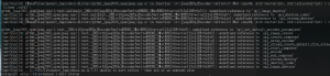
這將使用所選選項執行應用程式。-d 旗標會告訴程式用於推斷的裝置。-MYRIAD 利用 Intel® 類神經電腦棒 2啟動 MYRIAD 外掛程式。命令成功執行後,終端將顯示推斷的統計資料,並產生影像輸出。
INFO ] First inference took 267.43 ms
[Step 11/11] Dumping statistics report
Count: 12 iterations
Duration: 1620.69 ms
Latency:
Median: 532.82 ms
AVG: 494.30 ms
MIN: 278.83 ms
MAX: 557.00 ms
Throughput: 7.40 FPS
如果應用程式在您的Intel® NCS2上執行成功,OpenVINO™工具組和Intel® 類神經電腦棒 2已正確設定,以便在您的裝置上使用。
執行 benchmark_app Python 應用程式:
source ~/openvino_dist/setupvars.sh
cd ~/openvino/tools/benchmark_tool
python3 benchmark_app.py -i ~/Downloads/person.jpg -m ~/Downloads/person-vehicle-bike-detection-crossroad-0078.xml -d MYRIAD
如果應用程式在您的Intel® NCS2上成功執行,nGraph 模組將正確綁定至 Python。
環境變數
您必須更新多個環境變數,才能編譯並執行工具組應用程式OpenVINO。執行下列腳本以暫時設定環境變數:
source ~/openvino_dist/setupvars.sh
**(選用)** 關閉外殼時,會移除OpenVINO環境變數。作為一種選項,您可以永久設定環境變數如下:
echo “source ~/openvino_dist/setupvars.sh” >> ~/.bashrc
若要測試您的變更,請開啟新的終端。您將看到下列內容:
[setupvars.sh] OpenVINO environment initialized
這就完成了 Raspbian* 作業系統OpenVINO™工具組的開源分配建置程式,並以Intel® 類神經電腦棒 2方式使用。